Biomedical applications of small animal imaging are creating exciting opportunities to extend the scientific impact of visualization research. Specifically, the effective pairing of non-linear image filtering and direct volume rendering is one strategy for scientists to quickly explore and understand the volumetric scans of their specimens. Microscopic computed tomography imaging is an increasingly popular and powerful modality for small animal imaging. Here we highlight early work from collaborations at the University of Utah between the Scientific Computing and Imaging (SCI) Institute and the Department of Bioengineering, and between the SCI Institute and the Division of Pediatric Hematology-Oncology in the Department of Pediatrics. In the first instance, volume rendering provides information about the three-dimensional configuration of an electrode array implanted into the auditory nerve of a feline. In the second instance, volume rendering shows promise as a tool for visualizing bone tissue in the mouse embryo, although the signal-to-noise characteristics of the data require the use of sophisticated image pre-processing.
The data for both of these investigations was acquired with a General Electric EVS RS-9 computed tomography scanner at the University of Utah Small Animal Imaging Facility. The scanner generates 16-bit volumes roughly one gigabyte in size, with a spatial resolution of 21 x 21 x 21 microns.
Implanted Electrode Array
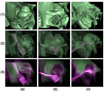 Fig. 1: Volume renderings of electrode array implanted in feline skull. The volume is rotated gradually upwards in columns (a), (b), and (c), from seeing the side of the cochlea exterior in (a), to looking down the path of the cochlear nerve in (c). From top to bottom, each row uses different rendering styles; (1): volume renderings with opaque bone; (2): volume renderings with translucent bone, showing the electrode leads in magenta; and summation projections of CT values (green) and gradient magnitudes (magenta). Fig. 1: Volume renderings of electrode array implanted in feline skull. The volume is rotated gradually upwards in columns (a), (b), and (c), from seeing the side of the cochlea exterior in (a), to looking down the path of the cochlear nerve in (c). From top to bottom, each row uses different rendering styles; (1): volume renderings with opaque bone; (2): volume renderings with translucent bone, showing the electrode leads in magenta; and summation projections of CT values (green) and gradient magnitudes (magenta). |
The feline auditory nerve itself is not discerned by CT imaging, but it is positioned at the center of the modiolus, the "bore" of the cochlea. Thus, the visualization task for this dataset is to determine whether the tips of the electrode array are correctly positioned with respect to the path of the nerve, as indicated by the surrounding bone surfaces. Because of the different radio-opacities of bone, air, and the electrode array, direct volume rendering provides a way of visualizing the objects in the dataset. (Fig. 1) In this case, the one-dimensional transfer functions which determine opacity and color were generated by inspecting a histogram of the CT values.
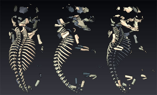
Non-Linear Filtering of Bone Scans
While visualization practitioners often consider CT datasets as being less noisy than other modalities such as ultrasound or clinical MRI, small animal imaging CT scans can present significant signal-to-noise challenges. One problem is with contrast: the tissues of interest do not always have markedly different radio-opacity than their surroundings. The developing bones of a mouse embryo, for example, are partially and unevenly calcified. Regions which consist solely of cartilage are essentially indistinguishable in their CT value from the nearby soft tissue. A related issue is that the size of some features can approach the limits of the imaging resolution. In combination with the effects of partial voluming, it can become difficult to distinguish CT values inside and outside small features. This hampers the creation of a meaningful visualization.Fig. 2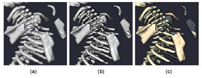 |
Fig. 3